Examples of space-based gravitational wave signal generation

EMRIs waveform

By running emri_demo.py script, a EMRIs waveform example is generated.

The default signal length is two years and default sampling rate is 10 seconds, and the generated waveform is saved at the same directory as test_EMRI.hdf5. You can adapt the configurations in emri_demo.py according to your own needs.

$ conda activate waveform
$ cd /workspace/GWAI/demos
$ python emri_demo.py
$ ls *EMRI*
test_EMRI.hdf5

To visulize the generated waveform, firstly you need to load the test_EMRI.hdf5 file.

>>> import h5py
>>> source = 'EMRI'
>>> f = h5py.File(f"test_{source}.hdf5", "r")
>>> all_keys = [key for key in f.keys()]
>>> d = f[all_keys[0]]
>>> print(f.filename, ":", all_keys)
>>> print(d.name, ":", d.shape)     # 10s sampling rate, 2-year-length waveform
>>> print(d[:])
test_EMRI.hdf5 : ['TDIdata']
/TDIdata : (4, 6311630)
[[ 0.00000000e+00  1.00000000e+01  2.00000000e+01 ...  6.31162720e+07
   6.31162800e+07  6.31162880e+07]
 [ 2.39214973e-21  2.85723663e-21  1.17999299e-21 ... -2.99196318e-21
  -5.15871471e-21  3.03701580e-21]
 [ 8.12895951e-21 -3.59335741e-21  7.26437602e-23 ... -1.12794030e-21
  -7.39320486e-21  3.79989830e-21]
 [ 4.23084649e-21  1.36245475e-21 -3.16980953e-21 ... -4.44047238e-21
   6.76437277e-21 -3.37023952e-21]]

Then by running plot_waveform.py, detailed information of the waveform is presented.

import matplotlib.pyplot as plt
from mpl_toolkits.axes_grid1.inset_locator import inset_axes
fig = plt.figure(figsize=(15,3), facecolor='white', dpi=100)
ax = fig.add_subplot(111)
ax.plot(d[0,:6000], d[1,:6000], alpha=0.8, label='X channel')
ax.plot(d[0,:6000], d[2,:6000], alpha=0.8, label='Y channel')
ax.plot(d[0,:6000], d[3,:6000], alpha=0.8, label='Z channel')
ax.legend(loc="lower right")
ax.set_xlabel('Time(s)')
ax.set_ylabel('Amplitude')
ax.set_title(f'{source} waveform')
axins = ax.inset_axes((0.2, 0.2, 0.4, 0.3))
pt = 500
axins.plot(d[0,:pt], d[1,:pt])
axins.plot(d[0,:pt], d[2,:pt])
axins.plot(d[0,:pt], d[3,:pt])
ax.indicate_inset_zoom(axins, alpha=0.8)
# plt.savefig(f'{source}_wave.png', dpi=100)
plt.show()

Source code, emri.png

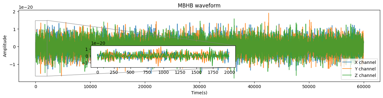
MBHB waveform

The MBHB waveform generation process is similar as EMRIs waveform. Hence, we only give a brief introduction here.

Generate waveform by running mbhb_demo.py.
Visulize the generated waveform by running plot_waveform.py (you only need to choose the corresponding GW source as shown below).

import h5py
# source = 'EMRI'
source = 'MBHB'
# source = 'SGWB'
# source = 'VGB'

Source code, mbhb.png

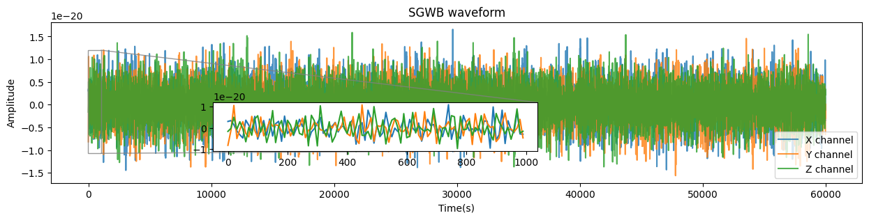
SGWB waveform

The SGWB waveform generation process is similar as EMRIs waveform. Hence, we only give a brief introduction here.

Generate waveform by running sgwb_demo.py.
Visulize the generated waveform by running plot_waveform.py (you only need to choose the corresponding GW source as shown below).

import h5py
# source = 'EMRI'
# source = 'MBHB'
source = 'SGWB'
# source = 'VGB'

Source code, sgwb.png

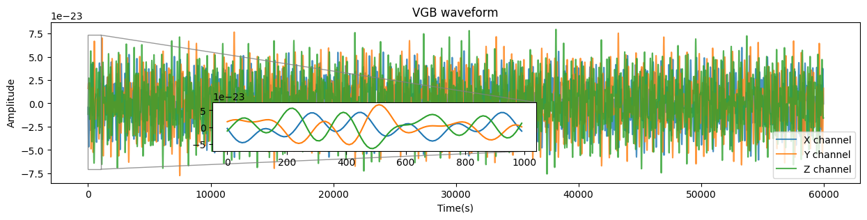
VGB waveform

The VGB waveform generation process is similar as EMRIs waveform. Hence, we only give a brief introduction here.

Generate waveform by running vgb_demo.py.
Visulize the generated waveform by running plot_waveform.py (you only need to choose the corresponding GW source as shown below).

import h5py
# source = 'EMRI'
# source = 'MBHB'
# source = 'SGWB'
source = 'VGB'

Source code, vgb.png